Vibration Modes in a T beam

4 minute read

Summary

This report investigates the vibrational response of T-beam structure, which can be regarded as a simplified aircraft fuselage tail-plane model. The first 6 natural frequencies of the structure will be determined. Assigned to us were individual tasks associated with the modelling of predicted mode shapes using theoretical principles. Each of the group members produced estimations of the respective mode shapes and derived a row of the flexibility matrix. The estimation methods were compared against each other to determine the best technique.

Introduction

Vibration is a topic that applies to a multitude of engineering applications. Developing an understanding through its theoretical and experimental analysis is vital. Across an abundance of industries the failure to mitigate against large energy transfers, with the correspondence of resonant frequencies, can result in the catastrophic failure/degradation of projects. An example of which is the Tacoma Narrows Suspension Bridge, in which wind induced vibrations led to oscillations at its fundamental mode and therefore the collapse of a multi-million dollar project.

This Vibrations lab revolves itself around experimentally testing and analysing the vibrational response of T-beam structure. Accelerometers recorded data over 32 points of the T-beam which was mechanically excited with a hammer. T-beam was approximated as a 6 degree of freedom model to give a basis of theoretical prediction. Each row of the flexibility matrix was calculated and the mass matrix of the T-beam was constructed. After the accumulation of data, Matlab codes were constructed to both predict and investigate the beams 6 mode shapes, Frequency Response Functions (FRF’s) and 6 natural frequencies.

Comparisons with in this report will be made between the predicted and experimental data. These will be justified using fundamental engineering principles that will help to validate/ invalidate the experimental data that was acquired. These engineering principles include the derivation of the equations of motion, the load sharing approach employed to construct the mass matrix, torsional effects present at the extremities of the beam and the eigenvalue problem used to evaluate the natural frequencies. These concepts will be investigated further in the sections to follow.

Theory

The vibration of the metal T beam outlined previously can be modeled using a Multiple Degree of Freedom system. Through employing a load sharing approach, with the associated mass distributions across the T beam, the flexibility matrix [a] and the dynamic matrix [D] can be calculated.

Equations of Motion

The equations of motion are required here to outline model the vibratory response of the T beam. They can be derived through 3 separate methods: Newton’s equation of motion, Lagrange’s method or through the use of the Stiffness and Flexibility influence coefficients. Newton’s method will be outlined with a 2 Degree of Freedom model to exhibit the consecutive stages of the derivation.

Each respective mass can be isolated the forces acting are equated.

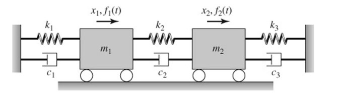
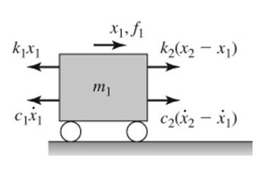
For the first mass newton’s second law of motion is applied with the external force f(t) applied.

Likewise for the second mass.

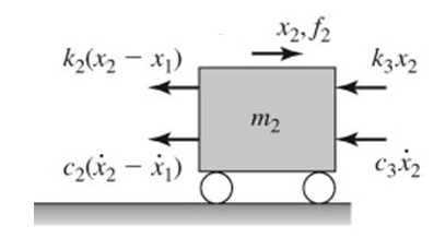
Combining the equations yields the following:

This is the equation of motion. Each matrix can be simplified to give the more commonly equation.

Where the derivatives of x are the acceleration vector, velocity vector respectively. x is the displacement vector and F is the force vector.

The Flexibility Matrix [K]

The viscous damping and force vector are set to zero within the T beam analysis. After inserting the mass matrix [M] for the beam, the stiffness matrix [k] must be obtained. The term k(ij) represents the force at point i due to a unit displacement at point j with all other points fixed. This term is the inverse of the “flexibility influence coefficient”.

[a] ([k]=〖[a]〗^(-1))

A term that eludes to the deflection at point i due to a unit force acting at point j (where the unit force is the only force acting). The flexibility coefficient is therefore calculated.

The technique adopted in calculating the flexibility coefficient varied between students. The most predominantly employed was the beam myosotis table.

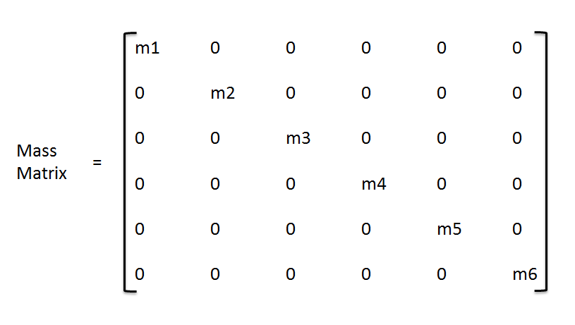
The Mass Matrix [M]

The mass matrix of the T beam was determined through attributing the beam into 6 points of mass, each with its individual degree of freedom. A technique described as the discritisation of a continuous system (or distributed parameter system).

After acquiring the density and respective areas for the beams the mass was assigned into its components necessary to form the matrix. A nodal point is assigned to the joint of the beam but is neglected in the formation of the mass matrix.

The nodal point mass distribution for the T beam is represented in the following two diagrams.

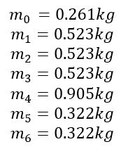
The mass breakdown for the specific T beam in question is as follows:

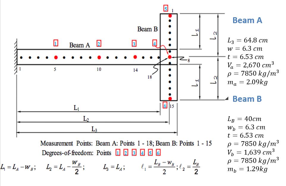
The mass of beam A was divided into 4 sub-sections, a quarter of the mass was attributed to node 1, 2 and 3. An eighth of the remaining mass was located at the support point of the cantilever ( m_(0 )) and the other eighth was assigned to the node point 4 (at an intersection with point B).

Likewise beam B was divided into 4 sub-sections.

One half of the mass was attributed to node point 4 (in addition to the contribution from A) and the remaining quarters assigned to nodes 5 & 6 at the extremities.

The overall Mass matrix is given as: